Multiobjective
Reference
SAS/OR example: https://go.documentation.sas.com/?cdcId=pgmsascdc&cdcVersion=9.4_3.4&docsetId=ormpug&docsetTarget=ormpug_lsosolver_examples07.htm&locale=en
SAS/OR code for example: http://support.sas.com/documentation/onlinedoc/or/ex_code/151/lsoe10.html
Model
import sasoptpy as so


def test(cas_conn, sols=False):

    m = so.Model(name='multiobjective', session=cas_conn)

    x = m.add_variables([1, 2], lb=0, ub=5, name='x')

    f1 = m.set_objective((x[1]-1)**2 + (x[1] - x[2])**2, name='f1', sense=so.MIN)
    f2 = m.append_objective((x[1]-x[2])**2 + (x[2] - 3)**2, name='f2', sense=so.MIN)

    m.solve(verbose=True, options={'with': 'blackbox', 'obj': (f1, f2), 'logfreq': 50})

    print('f1', f1.get_value())
    print('f2', f2.get_value())

    if sols:
        return dict(solutions=cas_conn.CASTable('allsols').to_frame(),
                    x=x, f1=f1, f2=f2)
    else:
        return f1.get_value()
Output
In [1]: import os

In [2]: hostname = os.getenv('CASHOST')

In [3]: port = os.getenv('CASPORT')

In [4]: from swat import CAS

In [5]: cas_conn = CAS(hostname, port)

In [6]: import sasoptpy
In [7]: from examples.client_side.multiobjective import test

In [8]: response = test(cas_conn, sols=True)
NOTE: Initialized model multiobjective.
NOTE: Added action set 'optimization'.
NOTE: Converting model multiobjective to OPTMODEL.
   var x {{1,2}} >= 0 <= 5;
   min f1 = (x[1] - 1) ^ (2) + (x[1] - x[2]) ^ (2);
   min f2 = (x[1] - x[2]) ^ (2) + (x[2] - 3) ^ (2);
   solve with blackbox obj (f1 f2) / logfreq=50;
   create data solution from [i]= {1.._NVAR_} var=_VAR_.name value=_VAR_ lb=_VAR_.lb ub=_VAR_.ub rc=_VAR_.rc;
   create data dual from [j] = {1.._NCON_} con=_CON_.name value=_CON_.body dual=_CON_.dual;
   create data allsols from [s]=(1.._NVAR_) name=_VAR_[s].name {j in 1.._NSOL_} <col('sol_'||j)=_VAR_[s].sol[j]>;

NOTE: Submitting OPTMODEL code to CAS server.
NOTE: Problem generation will use 8 threads.
NOTE: The problem has 2 variables (0 free, 0 fixed).
NOTE: The problem has 0 linear constraints (0 LE, 0 EQ, 0 GE, 0 range).
NOTE: The problem has 0 nonlinear constraints (0 LE, 0 EQ, 0 GE, 0 range).
NOTE: The OPTMODEL presolver removed 0 variables, 0 linear constraints, and 0 nonlinear constraints.
NOTE: The black-box solver is using up to 8 threads.
NOTE: The black-box solver is using the EAGLS optimizer algorithm.
NOTE: The problem has 2 variables (0 integer, 2 continuous).
NOTE: The problem has 0 constraints (0 linear, 0 nonlinear).
NOTE: The problem has 2 user-defined functions.
NOTE: The deterministic parallel mode is enabled.
           Iteration    Nondom        Progress    Infeasibility    Evals     Time
                   1         4               .                0       84        0
                  51       877       0.0000811                0     2876        0
                 101      1654       0.0000123                0     5576        1
                 151      2290  0.000003230545                0     8181        1
                 201      2874       0.0000182                0    10796        2
                 251      3422  0.000003148003                0    13447        3
                 301      3847  0.000001559509                0    16046        4
                 351      4282  0.000001159917                0    18733        5
                 401      4712  0.000002423148                0    21315        7
                 428      4932  0.000000704951                0    22734        8
NOTE: Function convergence criteria reached.
NOTE: The output table 'SOLUTION' in caslib 'CASUSER(casuser)' has 2 rows and 6 columns.
NOTE: The output table 'DUAL' in caslib 'CASUSER(casuser)' has 0 rows and 4 columns.
NOTE: The output table 'ALLSOLS' in caslib 'CASUSER(casuser)' has 2 rows and 4934 columns.
NOTE: The CAS table 'solutionSummary' in caslib 'CASUSER(casuser)' has 14 rows and 4 columns.
NOTE: The CAS table 'problemSummary' in caslib 'CASUSER(casuser)' has 12 rows and 4 columns.
f1 0.01497094056129493
f2 4.721632618656377
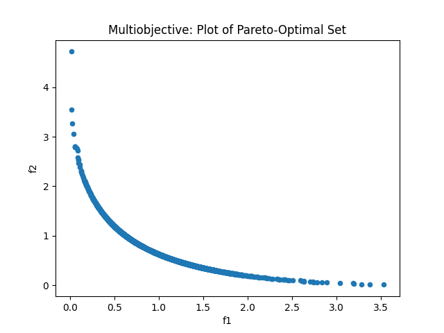
In [9]: import matplotlib.pyplot as plt

In [10]: sols = response['solutions']

In [11]: x = response['x']

In [12]: f1 = response['f1']

In [13]: f2 = response['f2']

In [14]: tr = sols.transpose()

In [15]: scvalues = tr.iloc[2:]

In [16]: scvalues = scvalues.astype({0: float, 1: float})

In [17]: x[1].set_value(scvalues[0])

In [18]: x[2].set_value(scvalues[1])

In [19]: scvalues['f1'] = f1.get_value()

In [20]: scvalues['f2'] = f2.get_value()

In [21]: f = scvalues.plot.scatter(x='f1', y='f2')

In [22]: f.set_title('Multiobjective: Plot of Pareto-Optimal Set');

In [23]: f
Out[23]: <matplotlib.axes._subplots.AxesSubplot at 0x7f06a2a0b4e0>