Workflows
sasoptpy can work with both client-side data and server-side data. Some limitations to the functionalities might apply in terms of which workflow is used. In this section, the overall flow of the package is explained.
Client-side models
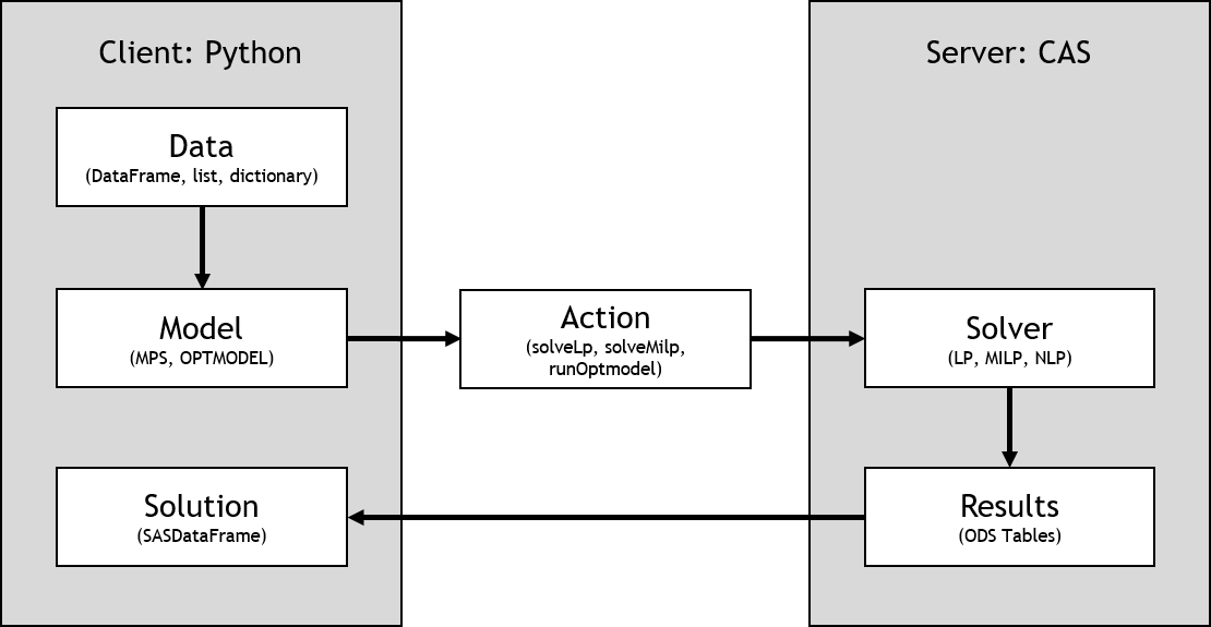
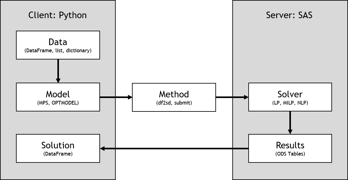
If the data are client-side (Python), then a concrete model is generated on the client and is uploaded by using one of the available CAS actions.
Using a client-side model brings several advantages, such as directly accessing variables, expressions, and constraints. You can more easily perform computationally intensive operations such as filtering data, sorting values, changing variable values, and printing expressions.
There are two main disadvantages of working with client-side models. First, if your model is relatively large, the generated MPS DataFrame or OPTMODEL code might allocate a large amount of memory on your machine. Second, the information that needs to be passed from client to server might be larger than it would be if you use a server-side model.
See the following representation of the client-side model workflow for CAS (Viya) servers:
See the following representation of the client-side model workflow for SAS clients:
Steps of modeling a simple knapsack problem are shown in the following subsections.
Reading data:
In [1]: import sasoptpy as so

In [2]: import pandas as pd

In [3]: from swat import CAS

In [4]: session = CAS(hostname, port)

In [5]: m = so.Model(name='client_CAS', session=session)
NOTE: Initialized model client_CAS.

In [6]: data = [
   ...:     ['clock', 8, 4, 3],
   ...:     ['mug', 10, 6, 5],
   ...:     ['headphone', 15, 7, 2],
   ...:     ['book', 20, 12, 10],
   ...:     ['pen', 1, 1, 15]
   ...:     ]
   ...:

In [7]: df = pd.DataFrame(data, columns=['item', 'value', 'weight', 'limit'])

In [8]: ITEMS = df.index

In [9]: value = df['value']

In [10]: weight = df['weight']

In [11]: limit = df['limit']

In [12]: total_weight = 55
In [13]: print(type(ITEMS), ITEMS)
<class 'pandas.core.indexes.range.RangeIndex'> RangeIndex(start=0, stop=5, step=1)
In [14]: print(type(total_weight), total_weight)
<class 'int'> 55
Here, you can obtain the column values one by one:
>>> df = df.set_index('item')
>>> ITEMS = df.index.tolist()
>>> value = df['value']
>>> weight = df['weight']
>>> limit = df['limit']
Creating the optimization model:
# Variables
In [15]: get = m.add_variables(ITEMS, name='get', vartype=so.INT, lb=0)

# Constraints
In [16]: m.add_constraints((get[i] <= limit[i] for i in ITEMS), name='limit_con');

In [17]: m.add_constraint(
   ....:     so.expr_sum(weight[i] * get[i] for i in ITEMS) <= total_weight,
   ....:     name='weight_con');
   ....:

# Objective
In [18]: total_value = so.expr_sum(value[i] * get[i] for i in ITEMS)

In [19]: m.set_objective(total_value, name='total_value', sense=so.MAX);

# Solve
In [20]: m.solve(verbose=True)
NOTE: Added action set 'optimization'.
NOTE: Converting model client_CAS to OPTMODEL.
   var get {{0,1,2,3,4}} integer >= 0;
   con limit_con_0 : get[0] <= 3;
   con limit_con_1 : get[1] <= 5;
   con limit_con_2 : get[2] <= 2;
   con limit_con_3 : get[3] <= 10;
   con limit_con_4 : get[4] <= 15;
   con weight_con : 4 * get[0] + 6 * get[1] + 7 * get[2] + 12 * get[3] + get[4] <= 55;
   max total_value = 8 * get[0] + 10 * get[1] + 15 * get[2] + 20 * get[3] + get[4];
   solve;
   create data solution from [i]= {1.._NVAR_} var=_VAR_.name value=_VAR_ lb=_VAR_.lb ub=_VAR_.ub rc=_VAR_.rc;
   create data dual from [j] = {1.._NCON_} con=_CON_.name value=_CON_.body dual=_CON_.dual;

NOTE: Submitting OPTMODEL code to CAS server.
NOTE: Problem generation will use 8 threads.
NOTE: The problem has 5 variables (0 free, 0 fixed).
NOTE: The problem has 0 binary and 5 integer variables.
NOTE: The problem has 6 linear constraints (6 LE, 0 EQ, 0 GE, 0 range).
NOTE: The problem has 10 linear constraint coefficients.
NOTE: The problem has 0 nonlinear constraints (0 LE, 0 EQ, 0 GE, 0 range).
NOTE: The OPTMODEL presolver is disabled for linear problems.
NOTE: The initial MILP heuristics are applied.
NOTE: The MILP presolver value AUTOMATIC is applied.
NOTE: The MILP presolver removed 0 variables and 5 constraints.
NOTE: The MILP presolver removed 5 constraint coefficients.
NOTE: The MILP presolver modified 0 constraint coefficients.
NOTE: The presolved problem has 5 variables, 1 constraints, and 5 constraint coefficients.
NOTE: The MILP solver is called.
NOTE: The parallel Branch and Cut algorithm is used.
NOTE: The Branch and Cut algorithm is using up to 8 threads.
             Node   Active   Sols    BestInteger      BestBound      Gap    Time
                0        1      4     99.0000000    199.0000000   50.25%       0
                0        1      4     99.0000000    102.3333333    3.26%       0
                0        1      4     99.0000000    102.3333333    3.26%       0
NOTE: The MILP presolver is applied again.
                0        1      4     99.0000000    102.3333333    3.26%       0
NOTE: Optimal.
NOTE: Objective = 99.
NOTE: The output table 'SOLUTION' in caslib 'CASUSER(casuser)' has 5 rows and 6 columns.
NOTE: The output table 'DUAL' in caslib 'CASUSER(casuser)' has 6 rows and 4 columns.
NOTE: The CAS table 'solutionSummary' in caslib 'CASUSER(casuser)' has 18 rows and 4 columns.
NOTE: The CAS table 'problemSummary' in caslib 'CASUSER(casuser)' has 20 rows and 4 columns.
Out[20]:
Selected Rows from Table SOLUTION

     i     var  value   lb             ub  rc
0  1.0  get[0]    2.0 -0.0  1.797693e+308 NaN
1  2.0  get[1]    5.0 -0.0  1.797693e+308 NaN
2  3.0  get[2]    2.0 -0.0  1.797693e+308 NaN
3  4.0  get[3]   -0.0 -0.0  1.797693e+308 NaN
4  5.0  get[4]    3.0 -0.0  1.797693e+308 NaN
You can display the generated OPTMODEL code at run time by using the
verbose=Trueoption. Here, you can see the coefficient values of the parameters inside the model.Parsing the results:
After the solve, the primal and dual solution tables are obtained. You can print the solution tables by using the
Model.get_solution()method.It is also possible to print the optimal solution by using the
get_solution_table()function.In [21]: print(m.get_solution()) Selected Rows from Table SOLUTION i var value lb ub rc 0 1.0 get[0] 2.0 -0.0 1.797693e+308 NaN 1 2.0 get[1] 5.0 -0.0 1.797693e+308 NaN 2 3.0 get[2] 2.0 -0.0 1.797693e+308 NaN 3 4.0 get[3] -0.0 -0.0 1.797693e+308 NaN 4 5.0 get[4] 3.0 -0.0 1.797693e+308 NaN
In [22]: print(so.get_solution_table(get, key=ITEMS))
   get
0  2.0
1  5.0
2  2.0
3 -0.0
4  3.0
In [23]: print('Total value:', total_value.get_value())
Total value: 99.0
Server-side models
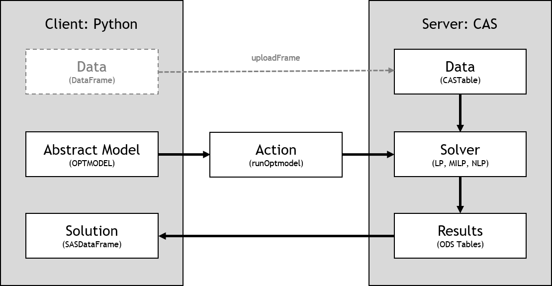
If the data are server-side (CAS or SAS), then an abstract model is generated on the client. This abstract model is later converted to PROC OPTMODEL code, which reads the data on the server.
The main advantage of the server-side models is faster upload times compared to client-side models. This is especially noticeable when using large numbers of variable and constraint groups.
The only disadvantage of using server-side models is that variables often need to be accessed directly from the resulting SASDataFrame objects. Because components of the models are abstract, accessing objects directly is often not possible.
See the following representation of the server-side model workflow for CAS (Viya) servers:
See the following representation of the server-side model workflow for SAS clients:

In the following steps, the same example is solved by using server-side data.
Creating the optimization model:
In [24]: from sasoptpy.actions import read_data

In [25]: m = so.Model(name='client_CAS', session=session)
NOTE: Initialized model client_CAS.
In [26]: cas_table = session.upload_frame(df, casout='data')
NOTE: Cloud Analytic Services made the uploaded file available as table DATA in caslib CASUSER(casuser).
NOTE: The table DATA has been created in caslib CASUSER(casuser) from binary data uploaded to Cloud Analytic Services.
In [27]: ITEMS = m.add_set(name='ITEMS', settype=so.STR)

In [28]: value = m.add_parameter(ITEMS, name='value')

In [29]: weight = m.add_parameter(ITEMS, name='weight')

In [30]: limit = m.add_parameter(ITEMS, name='limit')

In [31]: m.include(read_data(
   ....:    table=cas_table, index={'target':ITEMS, 'key': 'item'},
   ....:    columns=[value, weight, limit]))
   ....:

# Variables
In [32]: get = m.add_variables(ITEMS, name='get', vartype=so.INT, lb=0)

# Constraints
In [33]: m.add_constraints((get[i] <= limit[i] for i in ITEMS), name='limit_con');

In [34]: m.add_constraint(
   ....:     so.expr_sum(weight[i] * get[i] for i in ITEMS) <= total_weight,
   ....:     name='weight_con');
   ....:
# Objective
In [35]: total_value = so.expr_sum(value[i] * get[i] for i in ITEMS)

In [36]: m.set_objective(total_value, name='total_value', sense=so.MAX);

# Solve
In [37]: m.solve(verbose=True)
NOTE: Added action set 'optimization'.
NOTE: Converting model client_CAS to OPTMODEL.
   set <str> ITEMS;
   num value {{ITEMS}};
   num weight {{ITEMS}};
   num limit {{ITEMS}};
   read data DATA into ITEMS=[item] value weight limit;
   var get {{ITEMS}} integer >= 0;
   con limit_con {o37 in ITEMS} : get[o37] - limit[o37] <= 0;
   con weight_con : sum {i in ITEMS} (weight[i] * get[i]) <= 55;
   max total_value = sum {i in ITEMS} (value[i] * get[i]);
   solve;
   create data solution from [i]= {1.._NVAR_} var=_VAR_.name value=_VAR_ lb=_VAR_.lb ub=_VAR_.ub rc=_VAR_.rc;
   create data dual from [j] = {1.._NCON_} con=_CON_.name value=_CON_.body dual=_CON_.dual;

NOTE: Submitting OPTMODEL code to CAS server.
NOTE: There were 5 rows read from table 'DATA' in caslib 'CASUSER(casuser)'.
NOTE: Problem generation will use 8 threads.
NOTE: The problem has 5 variables (0 free, 0 fixed).
NOTE: The problem has 0 binary and 5 integer variables.
NOTE: The problem has 6 linear constraints (6 LE, 0 EQ, 0 GE, 0 range).
NOTE: The problem has 10 linear constraint coefficients.
NOTE: The problem has 0 nonlinear constraints (0 LE, 0 EQ, 0 GE, 0 range).
NOTE: The OPTMODEL presolver is disabled for linear problems.
NOTE: The initial MILP heuristics are applied.
NOTE: The MILP presolver value AUTOMATIC is applied.
NOTE: The MILP presolver removed 0 variables and 5 constraints.
NOTE: The MILP presolver removed 5 constraint coefficients.
NOTE: The MILP presolver modified 0 constraint coefficients.
NOTE: The presolved problem has 5 variables, 1 constraints, and 5 constraint coefficients.
NOTE: The MILP solver is called.
NOTE: The parallel Branch and Cut algorithm is used.
NOTE: The Branch and Cut algorithm is using up to 8 threads.
             Node   Active   Sols    BestInteger      BestBound      Gap    Time
                0        1      4     99.0000000    199.0000000   50.25%       0
                0        1      4     99.0000000    102.3333333    3.26%       0
                0        0      4     99.0000000     99.0000000    0.00%       0
NOTE: Optimal.
NOTE: Objective = 99.
NOTE: The output table 'SOLUTION' in caslib 'CASUSER(casuser)' has 5 rows and 6 columns.
NOTE: The output table 'DUAL' in caslib 'CASUSER(casuser)' has 6 rows and 4 columns.
NOTE: The CAS table 'solutionSummary' in caslib 'CASUSER(casuser)' has 18 rows and 4 columns.
NOTE: The CAS table 'problemSummary' in caslib 'CASUSER(casuser)' has 20 rows and 4 columns.
Out[37]:
Selected Rows from Table SOLUTION

     i             var  value   lb             ub  rc
0  1.0       get[book]    2.0 -0.0  1.797693e+308 NaN
1  2.0      get[clock]    3.0 -0.0  1.797693e+308 NaN
2  3.0  get[headphone]    2.0 -0.0  1.797693e+308 NaN
3  4.0        get[mug]   -0.0 -0.0  1.797693e+308 NaN
4  5.0        get[pen]    5.0 -0.0  1.797693e+308 NaN
Parsing the results:
# Print results
In [38]: print(m.get_solution())
Selected Rows from Table SOLUTION

     i             var  value   lb             ub  rc
0  1.0       get[book]    2.0 -0.0  1.797693e+308 NaN
1  2.0      get[clock]    3.0 -0.0  1.797693e+308 NaN
2  3.0  get[headphone]    2.0 -0.0  1.797693e+308 NaN
3  4.0        get[mug]   -0.0 -0.0  1.797693e+308 NaN
4  5.0        get[pen]    5.0 -0.0  1.797693e+308 NaN
In [39]: print('Total value:', m.get_objective_value())
Total value: 99.0
Because there is no direct access to expressions and variables, the optimal solution is printed by using the server response.
Limitations
In SAS Viya, nonlinear models can be solved only by using the runOptmodel action, which requires SAS Viya 3.4 or later.
User-defined decomposition blocks are available only in MPS mode, and therefore work only with client-side data.
Mixed usage (client-side and server-side data) might not work in some cases. A quick fix would be transferring the data in either direction.