Curve Fitting
Reference
SAS/OR example: http://go.documentation.sas.com/?docsetId=ormpex&docsetTarget=ormpex_ex11_toc.htm&docsetVersion=15.1&locale=en
SAS/OR code for example: http://support.sas.com/documentation/onlinedoc/or/ex_code/151/mpex11.html
Model
import sasoptpy as so
import pandas as pd


def test(cas_conn, sols=False):

    # Upload data to server first
    xy_raw = pd.DataFrame([
        [0.0, 1.0],
        [0.5, 0.9],
        [1.0, 0.7],
        [1.5, 1.5],
        [1.9, 2.0],
        [2.5, 2.4],
        [3.0, 3.2],
        [3.5, 2.0],
        [4.0, 2.7],
        [4.5, 3.5],
        [5.0, 1.0],
        [5.5, 4.0],
        [6.0, 3.6],
        [6.6, 2.7],
        [7.0, 5.7],
        [7.6, 4.6],
        [8.5, 6.0],
        [9.0, 6.8],
        [10.0, 7.3]
        ], columns=['x', 'y'])
    xy_data = cas_conn.upload_frame(xy_raw, casout={'name': 'xy_data',
                                                    'replace': True})

    # Read observations
    from sasoptpy.actions import read_data
    POINTS = so.Set(name='POINTS')
    x = so.ParameterGroup(POINTS, name='x')
    y = so.ParameterGroup(POINTS, name='y')
    read_st = read_data(
        table=xy_data,
        index={'target': POINTS, 'key': so.N},
        columns=[
            {'target': x, 'column': 'x'},
            {'target': y, 'column': 'y'}
        ]
    )

    # Parameters and variables
    order = so.Parameter(name='order')
    beta = so.VariableGroup(so.exp_range(0, order), name='beta')
    estimate = so.ImplicitVar(
        (beta[0] + so.expr_sum(beta[k] * x[i] ** k
                                for k in so.exp_range(1, order))
         for i in POINTS), name='estimate')

    surplus = so.VariableGroup(POINTS, name='surplus', lb=0)
    slack = so.VariableGroup(POINTS, name='slack', lb=0)

    objective1 = so.Expression(
        so.expr_sum(surplus[i] + slack[i] for i in POINTS), name='objective1')
    abs_dev_con = so.ConstraintGroup(
        (estimate[i] - surplus[i] + slack[i] == y[i] for i in POINTS),
        name='abs_dev_con')

    minmax = so.Variable(name='minmax')
    objective2 = so.Expression(minmax + 0.0, name='objective2')
    minmax_con = so.ConstraintGroup(
        (minmax >= surplus[i] + slack[i] for i in POINTS), name='minmax_con')

    order.set_init(1)
    L1 = so.Model(name='L1', session=cas_conn)
    L1.set_objective(objective1, sense=so.MIN, name='L1obj')
    L1.include(POINTS, x, y, read_st)
    L1.include(order, beta, estimate, surplus, slack, abs_dev_con)
    L1.add_postsolve_statement('print x y estimate surplus slack;')

    L1.solve(verbose=True)
    if sols:
        sol_data1 = L1.response['Print1.PrintTable'].sort_values('x')
        print(so.get_solution_table(beta))
        print(sol_data1.to_string())

    Linf = so.Model(name='Linf', session=cas_conn)
    Linf.include(L1, minmax, minmax_con)
    Linf.set_objective(objective2, sense=so.MIN, name='Linfobj')

    Linf.solve()
    if sols:
        sol_data2 = Linf.response['Print1.PrintTable'].sort_values('x')
        print(so.get_solution_table(beta))
        print(sol_data2.to_string())

    order.set_init(2)

    L1.solve()
    if sols:
        sol_data3 = L1.response['Print1.PrintTable'].sort_values('x')
        print(so.get_solution_table(beta))
        print(sol_data3.to_string())

    Linf.solve()
    if sols:
        sol_data4 = Linf.response['Print1.PrintTable'].sort_values('x')
        print(so.get_solution_table(beta))
        print(sol_data4.to_string())

    if sols:
        return (sol_data1, sol_data2, sol_data3, sol_data4)
    else:
        return Linf.get_objective_value()
Output
In [1]: import os

In [2]: hostname = os.getenv('CASHOST')

In [3]: port = os.getenv('CASPORT')

In [4]: from swat import CAS

In [5]: cas_conn = CAS(hostname, port)

In [6]: import sasoptpy
In [7]: from examples.server_side.curve_fitting import test

In [8]: (s1, s2, s3, s4) = test(cas_conn, sols=True)
NOTE: Cloud Analytic Services made the uploaded file available as table XY_DATA in caslib CASUSER(casuser).
NOTE: The table XY_DATA has been created in caslib CASUSER(casuser) from binary data uploaded to Cloud Analytic Services.
NOTE: Initialized model L1.
NOTE: Added action set 'optimization'.
NOTE: Converting model L1 to OPTMODEL.
   set POINTS;
   num x {POINTS};
   num y {POINTS};
   read data XY_DATA into POINTS=[_N_] x y;
   num order init 1;
   var beta {{0..order}};
   impvar estimate {o8 in POINTS} = beta[0] + sum {k in 1..order} (beta[k] * (x[o8]) ^ (k));
   var surplus {{POINTS}} >= 0;
   var slack {{POINTS}} >= 0;
   con abs_dev_con {o32 in POINTS} : y[o32] - estimate[o32] + surplus[o32] - slack[o32] = 0;
   min L1obj = sum {i in POINTS} (surplus[i] + slack[i]);
   solve;
   create data solution from [i]= {1.._NVAR_} var=_VAR_.name value=_VAR_ lb=_VAR_.lb ub=_VAR_.ub rc=_VAR_.rc;
   create data dual from [j] = {1.._NCON_} con=_CON_.name value=_CON_.body dual=_CON_.dual;
   print x y estimate surplus slack;

NOTE: Submitting OPTMODEL code to CAS server.
NOTE: There were 19 rows read from table 'XY_DATA' in caslib 'CASUSER(casuser)'.
NOTE: Problem generation will use 8 threads.
NOTE: The problem has 40 variables (2 free, 0 fixed).
NOTE: The problem uses 19 implicit variables.
NOTE: The problem has 19 linear constraints (0 LE, 19 EQ, 0 GE, 0 range).
NOTE: The problem has 75 linear constraint coefficients.
NOTE: The problem has 0 nonlinear constraints (0 LE, 0 EQ, 0 GE, 0 range).
NOTE: The OPTMODEL presolver is disabled for linear problems.
NOTE: The LP presolver value AUTOMATIC is applied.
NOTE: The LP presolver time is 0.03 seconds.
NOTE: The LP presolver removed 38 variables and 0 constraints.
NOTE: The LP presolver removed 38 constraint coefficients.
NOTE: The LP presolver formulated the dual of the problem.
NOTE: The presolved problem has 19 variables, 2 constraints, and 37 constraint coefficients.
NOTE: The LP solver is called.
NOTE: The Dual Simplex algorithm is used.
                              Objective
         Phase Iteration        Value         Time
          D 2          1    6.160000E+01         0
          D 2          5    1.146625E+01         0
NOTE: Optimal.
NOTE: Objective = 11.46625.
NOTE: The Dual Simplex solve time is 0.06 seconds.
NOTE: The output table 'SOLUTION' in caslib 'CASUSER(casuser)' has 40 rows and 6 columns.
NOTE: The output table 'DUAL' in caslib 'CASUSER(casuser)' has 19 rows and 4 columns.
NOTE: The CAS table 'solutionSummary' in caslib 'CASUSER(casuser)' has 13 rows and 4 columns.
NOTE: The CAS table 'problemSummary' in caslib 'CASUSER(casuser)' has 18 rows and 4 columns.
      beta
0  0.58125
1  0.63750
    COL1     x    y  estimate       surplus    slack
10  11.0   0.0  1.0   0.58125  0.000000e+00  0.41875
18  19.0   0.5  0.9   0.90000  5.551115e-17  0.00000
12  13.0   1.0  0.7   1.21875  5.187500e-01  0.00000
4    5.0   1.5  1.5   1.53750  3.750000e-02  0.00000
0    1.0   1.9  2.0   1.79250  0.000000e+00  0.20750
15  16.0   2.5  2.4   2.17500  0.000000e+00  0.22500
1    2.0   3.0  3.2   2.49375  0.000000e+00  0.70625
11  12.0   3.5  2.0   2.81250  8.125000e-01  0.00000
5    6.0   4.0  2.7   3.13125  4.312500e-01  0.00000
3    4.0   4.5  3.5   3.45000  0.000000e+00  0.05000
8    9.0   5.0  1.0   3.76875  2.768750e+00  0.00000
14  15.0   5.5  4.0   4.08750  8.750000e-02  0.00000
13  14.0   6.0  3.6   4.40625  8.062500e-01  0.00000
7    8.0   6.6  2.7   4.78875  2.088750e+00  0.00000
9   10.0   7.0  5.7   5.04375  0.000000e+00  0.65625
17  18.0   7.6  4.6   5.42625  8.262500e-01  0.00000
2    3.0   8.5  6.0   6.00000  0.000000e+00  0.00000
6    7.0   9.0  6.8   6.31875  0.000000e+00  0.48125
16  17.0  10.0  7.3   6.95625  0.000000e+00  0.34375
NOTE: Initialized model Linf.
NOTE: Added action set 'optimization'.
NOTE: Converting model Linf to OPTMODEL.
NOTE: Submitting OPTMODEL code to CAS server.
NOTE: There were 19 rows read from table 'XY_DATA' in caslib 'CASUSER(casuser)'.
NOTE: Problem generation will use 8 threads.
NOTE: The problem has 41 variables (3 free, 0 fixed).
NOTE: The problem uses 19 implicit variables.
NOTE: The problem has 38 linear constraints (0 LE, 19 EQ, 19 GE, 0 range).
NOTE: The problem has 132 linear constraint coefficients.
NOTE: The problem has 0 nonlinear constraints (0 LE, 0 EQ, 0 GE, 0 range).
NOTE: The OPTMODEL presolver is disabled for linear problems.
NOTE: The LP presolver value AUTOMATIC is applied.
NOTE: The LP presolver time is 0.00 seconds.
NOTE: The LP presolver removed 0 variables and 0 constraints.
NOTE: The LP presolver removed 0 constraint coefficients.
NOTE: The presolved problem has 41 variables, 38 constraints, and 132 constraint coefficients.
NOTE: The LP solver is called.
NOTE: The Dual Simplex algorithm is used.
                              Objective
         Phase Iteration        Value         Time
          D 2          1   -1.900000E+00         0
          P 2         26    1.725000E+00         0
NOTE: Optimal.
NOTE: Objective = 1.725.
NOTE: The Dual Simplex solve time is 0.01 seconds.
NOTE: The output table 'SOLUTION' in caslib 'CASUSER(casuser)' has 41 rows and 6 columns.
NOTE: The output table 'DUAL' in caslib 'CASUSER(casuser)' has 38 rows and 4 columns.
NOTE: The CAS table 'solutionSummary' in caslib 'CASUSER(casuser)' has 13 rows and 4 columns.
NOTE: The CAS table 'problemSummary' in caslib 'CASUSER(casuser)' has 18 rows and 4 columns.
    beta
0 -0.400
1  0.625
    COL1     x    y  estimate  surplus   slack
10  11.0   0.0  1.0   -0.4000    0.000  1.4000
18  19.0   0.5  0.9   -0.0875    0.000  0.9875
12  13.0   1.0  0.7    0.2250    0.000  0.4750
4    5.0   1.5  1.5    0.5375    0.000  0.9625
0    1.0   1.9  2.0    0.7875    0.000  1.2125
15  16.0   2.5  2.4    1.1625    0.000  1.2375
1    2.0   3.0  3.2    1.4750    0.000  1.7250
11  12.0   3.5  2.0    1.7875    0.000  0.2125
5    6.0   4.0  2.7    2.1000    0.000  0.6000
3    4.0   4.5  3.5    2.4125    0.000  1.0875
8    9.0   5.0  1.0    2.7250    1.725  0.0000
14  15.0   5.5  4.0    3.0375    0.000  0.9625
13  14.0   6.0  3.6    3.3500    0.000  0.2500
7    8.0   6.6  2.7    3.7250    1.025  0.0000
9   10.0   7.0  5.7    3.9750    0.000  1.7250
17  18.0   7.6  4.6    4.3500    0.000  0.2500
2    3.0   8.5  6.0    4.9125    0.000  1.0875
6    7.0   9.0  6.8    5.2250    0.000  1.5750
16  17.0  10.0  7.3    5.8500    0.000  1.4500
NOTE: Added action set 'optimization'.
NOTE: Converting model L1 to OPTMODEL.
NOTE: Submitting OPTMODEL code to CAS server.
NOTE: There were 19 rows read from table 'XY_DATA' in caslib 'CASUSER(casuser)'.
NOTE: Problem generation will use 8 threads.
NOTE: The problem has 41 variables (3 free, 0 fixed).
NOTE: The problem uses 19 implicit variables.
NOTE: The problem has 19 linear constraints (0 LE, 19 EQ, 0 GE, 0 range).
NOTE: The problem has 93 linear constraint coefficients.
NOTE: The problem has 0 nonlinear constraints (0 LE, 0 EQ, 0 GE, 0 range).
NOTE: The OPTMODEL presolver is disabled for linear problems.
NOTE: The LP presolver value AUTOMATIC is applied.
NOTE: The LP presolver time is 0.00 seconds.
NOTE: The LP presolver removed 38 variables and 0 constraints.
NOTE: The LP presolver removed 38 constraint coefficients.
NOTE: The LP presolver formulated the dual of the problem.
NOTE: The presolved problem has 19 variables, 3 constraints, and 55 constraint coefficients.
NOTE: The LP solver is called.
NOTE: The Dual Simplex algorithm is used.
                              Objective
         Phase Iteration        Value         Time
          D 2          1    6.160000E+01         0
          D 2          5    1.045896E+01         0
NOTE: Optimal.
NOTE: Objective = 10.458964706.
NOTE: The Dual Simplex solve time is 0.01 seconds.
NOTE: The output table 'SOLUTION' in caslib 'CASUSER(casuser)' has 41 rows and 6 columns.
NOTE: The output table 'DUAL' in caslib 'CASUSER(casuser)' has 19 rows and 4 columns.
NOTE: The CAS table 'solutionSummary' in caslib 'CASUSER(casuser)' has 13 rows and 4 columns.
NOTE: The CAS table 'problemSummary' in caslib 'CASUSER(casuser)' has 18 rows and 4 columns.
       beta
0  0.982353
1  0.294510
2  0.033725
    COL1     x    y  estimate       surplus     slack
10  11.0   0.0  1.0  0.982353  0.000000e+00  0.017647
18  19.0   0.5  0.9  1.138039  2.380392e-01  0.000000
12  13.0   1.0  0.7  1.310588  6.105882e-01  0.000000
4    5.0   1.5  1.5  1.500000 -6.938894e-17  0.000000
0    1.0   1.9  2.0  1.663671  0.000000e+00  0.336329
15  16.0   2.5  2.4  1.929412  0.000000e+00  0.470588
1    2.0   3.0  3.2  2.169412  0.000000e+00  1.030588
11  12.0   3.5  2.0  2.426275  4.262745e-01  0.000000
5    6.0   4.0  2.7  2.700000 -1.110223e-16  0.000000
3    4.0   4.5  3.5  2.990588  0.000000e+00  0.509412
8    9.0   5.0  1.0  3.298039  2.298039e+00  0.000000
14  15.0   5.5  4.0  3.622353  0.000000e+00  0.377647
13  14.0   6.0  3.6  3.963529  3.635294e-01  0.000000
7    8.0   6.6  2.7  4.395200  1.695200e+00  0.000000
9   10.0   7.0  5.7  4.696471  0.000000e+00  1.003529
17  18.0   7.6  4.6  5.168612  5.686118e-01  0.000000
2    3.0   8.5  6.0  5.922353  0.000000e+00  0.077647
6    7.0   9.0  6.8  6.364706  0.000000e+00  0.435294
16  17.0  10.0  7.3  7.300000  4.440892e-16  0.000000
NOTE: Added action set 'optimization'.
NOTE: Converting model Linf to OPTMODEL.
NOTE: Submitting OPTMODEL code to CAS server.
NOTE: There were 19 rows read from table 'XY_DATA' in caslib 'CASUSER(casuser)'.
NOTE: Problem generation will use 8 threads.
NOTE: The problem has 42 variables (4 free, 0 fixed).
NOTE: The problem uses 19 implicit variables.
NOTE: The problem has 38 linear constraints (0 LE, 19 EQ, 19 GE, 0 range).
NOTE: The problem has 150 linear constraint coefficients.
NOTE: The problem has 0 nonlinear constraints (0 LE, 0 EQ, 0 GE, 0 range).
NOTE: The OPTMODEL presolver is disabled for linear problems.
NOTE: The LP presolver value AUTOMATIC is applied.
NOTE: The LP presolver time is 0.00 seconds.
NOTE: The LP presolver removed 0 variables and 0 constraints.
NOTE: The LP presolver removed 0 constraint coefficients.
NOTE: The presolved problem has 42 variables, 38 constraints, and 150 constraint coefficients.
NOTE: The LP solver is called.
NOTE: The Dual Simplex algorithm is used.
                              Objective
         Phase Iteration        Value         Time
          D 2          1   -1.900000E+00         0
          P 2         29    1.475000E+00         0
NOTE: Optimal.
NOTE: Objective = 1.475.
NOTE: The Dual Simplex solve time is 0.01 seconds.
NOTE: The output table 'SOLUTION' in caslib 'CASUSER(casuser)' has 42 rows and 6 columns.
NOTE: The output table 'DUAL' in caslib 'CASUSER(casuser)' has 38 rows and 4 columns.
NOTE: The CAS table 'solutionSummary' in caslib 'CASUSER(casuser)' has 13 rows and 4 columns.
NOTE: The CAS table 'problemSummary' in caslib 'CASUSER(casuser)' has 18 rows and 4 columns.
    beta
0  2.475
1 -0.625
2  0.125
    COL1     x    y  estimate   surplus     slack
10  11.0   0.0  1.0   2.47500  1.475000  0.000000
18  19.0   0.5  0.9   2.19375  1.293750  0.000000
12  13.0   1.0  0.7   1.97500  1.275000  0.000000
4    5.0   1.5  1.5   1.81875  0.318750  0.000000
0    1.0   1.9  2.0   1.73875  0.606875  0.868125
15  16.0   2.5  2.4   1.69375  0.000000  0.706250
1    2.0   3.0  3.2   1.72500  0.000000  1.475000
11  12.0   3.5  2.0   1.81875  0.000000  0.181250
5    6.0   4.0  2.7   1.97500  0.000000  0.725000
3    4.0   4.5  3.5   2.19375  0.000000  1.306250
8    9.0   5.0  1.0   2.47500  1.475000  0.000000
14  15.0   5.5  4.0   2.81875  0.000000  1.181250
13  14.0   6.0  3.6   3.22500  0.000000  0.375000
7    8.0   6.6  2.7   3.79500  1.095000  0.000000
9   10.0   7.0  5.7   4.22500  0.000000  1.475000
17  18.0   7.6  4.6   4.94500  0.345000  0.000000
2    3.0   8.5  6.0   6.19375  0.193750  0.000000
6    7.0   9.0  6.8   6.97500  0.175000  0.000000
16  17.0  10.0  7.3   8.72500  1.425000  0.000000
# Plots
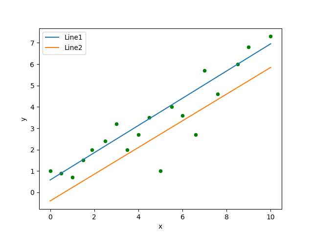
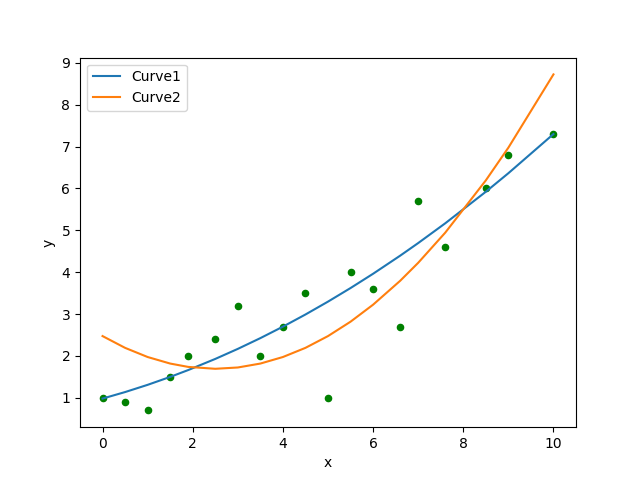
In [1]: import matplotlib.pyplot as plt
In [2]: p1 = s1.plot.scatter(x='x', y='y', c='g')
In [3]: s1.plot.line(ax=p1, x='x', y='estimate', label='Line1');
In [4]: s2.plot.line(ax=p1, x='x', y='estimate', label='Line2');
In [5]: p1
Out[5]: <matplotlib.axes._subplots.AxesSubplot at 0x7f06d1c95940>
In [6]: p2 = s3.plot.scatter(x='x', y='y', c='g')
In [7]: s3.plot.line(ax=p2, x='x', y='estimate', label='Curve1');
In [8]: s4.plot.line(ax=p2, x='x', y='estimate', label='Curve2');
In [9]: p2
Out[9]: <matplotlib.axes._subplots.AxesSubplot at 0x7f06ac12a6d8>