Getting Started
To connect to an ESP server, you just need a hostname and port number.
These are passed to the ESP constructor.
In [1]: import esppy

In [2]: conn = esppy.ESP(host, port)

In [3]: conn
Out[3]: ESP('http://lax95d01.unx.sas.com:40012')
Server Introspection
Once connected, we can query the server for basic information about the server itself, as well as projects in the server.
In [4]: conn.server_info
Out[4]:
{'version': '7.1',
 'engine': '04f125da-b540-4b71-96ea-b3200d5dc401',
 'analytics-license': True,
 'primary-server': True,
 'pubsub': 40011,
 'http': 40012}
We don’t have any projects loaded in the server yet, so the following will just return an empty dictionary.
In [5]: conn.get_projects()
Out[5]: {}
In [6]: conn.get_windows()
Out[6]: {}
Loading a Project
We’ll start off by loading a simple project from an XML project definition. The XML is shown below.
In [7]: proj_xml = '''
   ...: <engine>
   ...:   <projects>
   ...:     <project name='project' pubsub='auto' threads='1' use-tagged-token='true'>
   ...:       <contqueries>
   ...:         <contquery name='contquery' trace='w_data w_calculate'>
   ...:           <windows>
   ...:             <window-source name='w_data' insert-only='true'>
   ...:               <schema>
   ...:                 <fields>
   ...:                   <field name='id'   type='int64' key='true'/>
   ...:                   <field name='time' type='double'/>
   ...:                   <field name='x'    type='double'/>
   ...:                   <field name='y'    type='double'/>
   ...:                   <field name='z'    type='double'/>
   ...:                 </fields>
   ...:               </schema>
   ...:             </window-source>
   ...:             <window-source name='w_request' insert-only='true'>
   ...:               <schema>
   ...:                 <fields>
   ...:                   <field name='req_id'  type='int64' key='true'/>
   ...:                   <field name='req_key' type='string'/>
   ...:                   <field name='req_val' type='string'/>
   ...:                 </fields>
   ...:               </schema>
   ...:             </window-source>
   ...:             <window-calculate name='w_calculate' algorithm='Summary'>
   ...:               <schema>
   ...:                 <fields>
   ...:                   <field name='id'     type='int64' key='true'/>
   ...:                   <field name='x'      type='double'/>
   ...:                   <field name='mean_x' type='double'/>
   ...:                   <field name='n_x'    type='int64'/>
   ...:                 </fields>
   ...:               </schema>
   ...:               <parameters>
   ...:                 <properties>
   ...:                   <property name="windowLength">5</property>
   ...:                 </properties>
   ...:               </parameters>
   ...:               <input-map>
   ...:                 <properties>
   ...:                   <property name="input">x</property>
   ...:                 </properties>
   ...:               </input-map>
   ...:               <output-map>
   ...:                 <properties>
   ...:                   <property name="meanOut">mean_x</property>
   ...:                   <property name="nOut">n_x</property>
   ...:                 </properties>
   ...:               </output-map>
   ...:             </window-calculate>
   ...:           </windows>
   ...:           <edges>
   ...:             <edge source='w_data'    target='w_calculate' role='data'/>
   ...:             <edge source='w_request' target='w_calculate' role='request'/>
   ...:           </edges>
   ...:         </contquery>
   ...:       </contqueries>
   ...:     </project>
   ...:   </projects>
   ...: </engine>
   ...: '''
   ...:
In this project definition, we have a project named “project”, a single continuous query named ‘contquery’, and three windows named ‘w_data’, ‘w_request’, and ‘w_calculate’. w_data and w_request are data source windows, and w_calculate is a calculation window that is computing the mean and total count of the x variable. The mean of x is computed over a window of length 5.
To load the project definition into the server, you use the load_project()
method of the connection.
In [8]: walk = conn.load_project(proj_xml)
A diagram of the project is shown below. This diagram will be displayed in a Jupyter notebook if the last line of your code cell returns a project object. Note that if you only have a single continuous query object named ‘contquery’ (which is the default), it will not be displayed in the diagram.

You can also display all of the window schemas by using the schema=True
option of the Project.to_graph() method.
In [9]: walk.to_graph(schema=True)
Out[9]: <graphviz.dot.Digraph at 0x1fc07f55278>

While we are passing in an XML string here to load the project, the
load_project() also accepts filenames, file-like objects, or
Project objects (as we will see later on).
Now that we have a project loaded, we’ll see that the ESP.get_projects()
method now returns a dictionary with one entry.
In [10]: conn.get_projects()
Out[10]: {'project': Project(name='project')}
We can also get all of the windows configured in the server, or in the project.
In [11]: conn.get_windows()
Out[11]:
{'project.contquery.w_calculate': CalculateWindow(name='w_calculate', contquery='contquery', project='project'),
 'project.contquery.w_data': SourceWindow(name='w_data', contquery='contquery', project='project'),
 'project.contquery.w_request': SourceWindow(name='w_request', contquery='contquery', project='project')}

In [12]: walk.get_windows()
Out[12]:
{'w_calculate': CalculateWindow(name='w_calculate', contquery='contquery', project='project'),
 'w_data': SourceWindow(name='w_data', contquery='contquery', project='project'),
 'w_request': SourceWindow(name='w_request', contquery='contquery', project='project')}
Windows in the default continuous query can be accessed in the project’s windows attribute.
In [13]: walk.windows
Out[13]: {'w_data': SourceWindow(name='w_data', contquery='contquery', project='project'), 'w_request': SourceWindow(name='w_request', contquery='contquery', project='project'), 'w_calculate': CalculateWindow(name='w_calculate', contquery='contquery', project='project')}
In [14]: walk.windows['w_data']
Out[14]: SourceWindow(name='w_data', contquery='contquery', project='project')
These objects can also be displayed as diagrams in Jupyter or by using
the to_graph() method directly to generate SVG.
In [15]: walk.windows['w_data'].to_graph(schema=True)
Out[15]: <graphviz.dot.Digraph at 0x1fc080d74a8>

Working with Windows
The windows within a project are where most of the action occurs. Data streams into and out of windows, some windows will do calculations, others are used to train models and score streams of data.
In addition to the server-side processing of windows, the client-side also has many features of interacting with windows. Windows on the client act like streaming DataFrames. They can be configured to cache events from the server and DataFrame operations can be applied to the cached data.
We’ll begin by getting a reference to our data and calculation windows.
In [16]: w_data = walk.windows['w_data']

In [17]: w_calc = walk.windows['w_calculate']
Now that we have these Window objects, we can interact with them. Let’s
begin by injecting some data into the w_data window. The easiest way to
inject data into a window is by using the Window.publish_events() method.
This uses a websocket to insert data events into a window. The data can be
a string containing CSV, JSON, or XML data, a file-like object containing
CSV, JSON, or XML data, or a DataFrame.
For this example, we’ll use the following CSV data.
In [18]: walk_data = '''1,0,0.69464,3.1735,7.5048
   ....:     2,0.030639,0.14982,3.4868,9.2755
   ....:     3,0.069763,-0.29965,1.9477,9.112
   ....:     4,0.099823,-1.6889,1.4165,10.12
   ....:     5,0.12982,-2.1793,0.95342,10.924
   ....:     6,0.15979,-2.3018,0.23155,10.651
   ....:     7,0.18982,-1.4165,1.185,11.073
   ....:     8,0.2204,-0.27241,2.2201,11.986
   ....:     9,0.24976,-0.61292,2.2201,11.986
   ....:     10,0.27972,1.3348,4.2495,11.414
   ....:     11,0.31802,3.4459,7.5865,12.599
   ....:     12,0.34976,1.4982,4.9033,10.692
   ....:     13,0.37985,-1.7979,1.1169,9.9156
   ....:     14,0.40976,-2.3699,0.10896,9.003
   ....:     15,0.44983,-1.4982,2.3427,9.2346
   ....:     16,0.4798,-0.34051,3.2144,8.2403
   ....:     17,0.50977,-0.23155,2.4925,8.4991
   ....:     18,0.53979,-0.53119,1.5391,9.1529
   ....:     19,0.56976,-1.5663,1.0351,10.801
   ....:     20,0.59979,-1.5255,1.2258,11.346
   ....:     21,0.62979,-0.88532,2.9148,9.7249
   ....:     22,0.65982,-1.3076,2.3699,9.4253
   ....:     23,0.68979,-0.65378,2.8739,8.9622
   ....:     24,0.72055,0.23155,3.909,9.507
   ....:     25,0.75009,-0.42223,2.6423,9.8475
   ....:     26,0.78116,-0.57205,2.4925,9.1937
   ....:     27,0.80984,-0.65378,3.4459,8.0088
   ....:     28,0.83987,-0.34051,3.5277,9.112
   ....:     29,0.86981,-0.34051,3.1463,9.7249
   ....:     30,0.89978,-0.84446,3.2144,9.2346
   ....:     31,0.92978,-1.0351,3.1463,9.5342
   ....:     32,0.9599,-1.1169,2.8739,10.038
   ....:     33,0.98984,-1.2258,3.5277,9.2346
   ....:     34,1.0199,-1.0351,3.5958,8.8124
   ....:     35,1.0498,-0.8036,3.7184,9.1529
   ....:     36,1.0797,-0.72188,3.8273,8.9622
   ....:     37,1.1098,-1.185,3.4051,8.431
   ....:     38,1.1399,-1.6072,3.4051,8.7715
   ....:     39,1.1699,-1.7298,3.4868,9.0848
   ....:     40,1.1997,-1.757,3.6366,8.6898
   ....:     41,1.2298,-1.757,3.9908,8.8532
   ....:     42,1.2599,-1.9205,4.1406,8.8124
   ....:     43,1.2903,-1.8387,4.0589,8.8124
   ....:     44,1.3198,-1.7298,3.7184,8.54
   ....:     45,1.3513,-1.757,3.8682,8.3084
   ....:     46,1.3799,-1.757,3.7592,8.6625
   ....:     47,1.4098,-1.757,3.6775,8.7306
   ....:     48,1.4398,-1.9205,3.8682,9.1937
   ....:     49,1.4698,-1.757,4.0589,9.0439
   ....:     50,1.4998,-1.5663,4.1814,8.7306
   ....: '''
   ....:
The columns in this data set are id, time, x, y, and z
which corresponds to the schema in the w_data window. To inject the
events we call the publish_events() with the above string. We can also
control the rate at which the events appear in the window. We will specify
pause=500 to set the event rate to one event for every 500 milliseconds.
In [19]: w_data.publish_events(walk_data, pause=500)
Now that we have data flowing into the window, we can start event
processing on the client using the subscribe() method.
In [20]: w_data.subscribe()
After a few seconds, we should have some data being cached locally.
In [21]: w_data
Out[21]:
        time        x        y        z
id
2   0.030639  0.14982  3.48680   9.2755
3   0.069763 -0.29965  1.94770   9.1120
4   0.099823 -1.68890  1.41650  10.1200
5   0.129820 -2.17930  0.95342  10.9240
6   0.159790 -2.30180  0.23155  10.6510
7   0.189820 -1.41650  1.18500  11.0730
By default, windows will accumulate events indefinitely. You can control
the number of cached events and the length of time that events are processed
using the limit and horizon arguments.
The limit argument sets the maximum number of rows of
event data that are stored locally. The horizon argument
specifies either the amount of time that events should be processed, or
the total number of events that should be processed, or both. Let’s look
at examples of each of them.
The limit Argument
Setting the limit argument in the subscribe method, limits the number of
rows of event data that are cached to that value. Let’s set limit=7.
In [22]: w_data.subscribe(limit=7)
We now see that we only have 7 rows of data locally cached.
In [23]: w_data
Out[23]:
       time        x        y        z
id
9   0.24976 -0.61292  2.22010  11.9860
10  0.27972  1.33480  4.24950  11.4140
11  0.31802  3.44590  7.58650  12.5990
12  0.34976  1.49820  4.90330  10.6920
13  0.37985 -1.79790  1.11690   9.9156
14  0.40976 -2.36990  0.10896   9.0030
15  0.44983 -1.49820  2.34270   9.2346
The horizon Argument
The horizon argument takes several types of values:
- datetime.datetime
Specifies a date and time when event processing should stop
- datetime.date
Specifies a date when event processing should stop
- datetime.time
Specifies a time when event processing should stop
- datetime.timedelta
Specifies a duration of time that event processing should happen
- int
Specifies a total number of events to process before stopping
- string
Specifies an expression based on the variables in the event that, when True, stops event processing
In addition, a tuple of any of the types above can be specified. In this case, if any of the elements of the tuple indicate that event processing should end, event processing stops. Let’s look at an example.
In [24]: import time

In [25]: import datetime

In [26]: w_data.subscribe(horizon=datetime.timedelta(seconds=3))

# Events should still be processing
In [27]: print(w_data)
Empty DataFrame
Columns: [time, x, y, z]
Index: []

# After 4 seconds, no more events should be processed
In [28]: time.sleep(4)

In [29]: print(w_data)
       time        x       y        z
id
17  0.50977 -0.23155  2.4925   8.4991
18  0.53979 -0.53119  1.5391   9.1529
19  0.56976 -1.56630  1.0351  10.8010
20  0.59979 -1.52550  1.2258  11.3460
21  0.62979 -0.88532  2.9148   9.7249

# Again, the local cache of data should be the same
In [30]: time.sleep(2)

In [31]: print(w_data)
       time        x       y        z
id
17  0.50977 -0.23155  2.4925   8.4991
18  0.53979 -0.53119  1.5391   9.1529
19  0.56976 -1.56630  1.0351  10.8010
20  0.59979 -1.52550  1.2258  11.3460
21  0.62979 -0.88532  2.9148   9.7249
Rather than using a deadline, let’s set an expression that will end
our data collection. In this case, when the time column is above
1.0, our event collection will end. In addition, we can add an absolute
event count of 100 to stop event processing if the expression never
becomes true and we want to stop event processing after 100 total events.
In [32]: w_data.subscribe(horizon=('time > 1.0', 100))

In [33]: print(w_data)
Empty DataFrame
Columns: [time, x, y, z]
Index: []

# After 4 seconds, time should be > 1.0
In [34]: time.sleep(4)

In [35]: print(w_data)
       time        x       y        z
id
29  0.86981 -0.34051  3.1463   9.7249
30  0.89978 -0.84446  3.2144   9.2346
31  0.92978 -1.03510  3.1463   9.5342
32  0.95990 -1.11690  2.8739  10.0380
33  0.98984 -1.22580  3.5277   9.2346

# Again, the local cache of data should be the same
In [36]: time.sleep(4)

In [37]: print(w_data)
       time        x       y        z
id
29  0.86981 -0.34051  3.1463   9.7249
30  0.89978 -0.84446  3.2144   9.2346
31  0.92978 -1.03510  3.1463   9.5342
32  0.95990 -1.11690  2.8739  10.0380
33  0.98984 -1.22580  3.5277   9.2346
Now that we know how to inject data into an ESP window and process the resulting events, we can look at how to use window objects as DataFrames.
Using Windows as DataFrames
As we saw in the previous section, the data in a window prints out much like
a pandas.DataFrame would. It is possible to access any DataFrame
attribute or method on an ESP window. The accessing of DataFrame attributes and
methods on a window object are simply passed through to the underlying
data store.
For example, to get basic information about the data in the window, we can
use the info method.
In [38]: w_data.info()
<class 'pandas.core.frame.DataFrame'>
Int64Index: 5 entries, 29 to 33
Data columns (total 4 columns):
time    5 non-null float64
x       5 non-null float64
y       5 non-null float64
z       5 non-null float64
dtypes: float64(4)
memory usage: 200.0 bytes
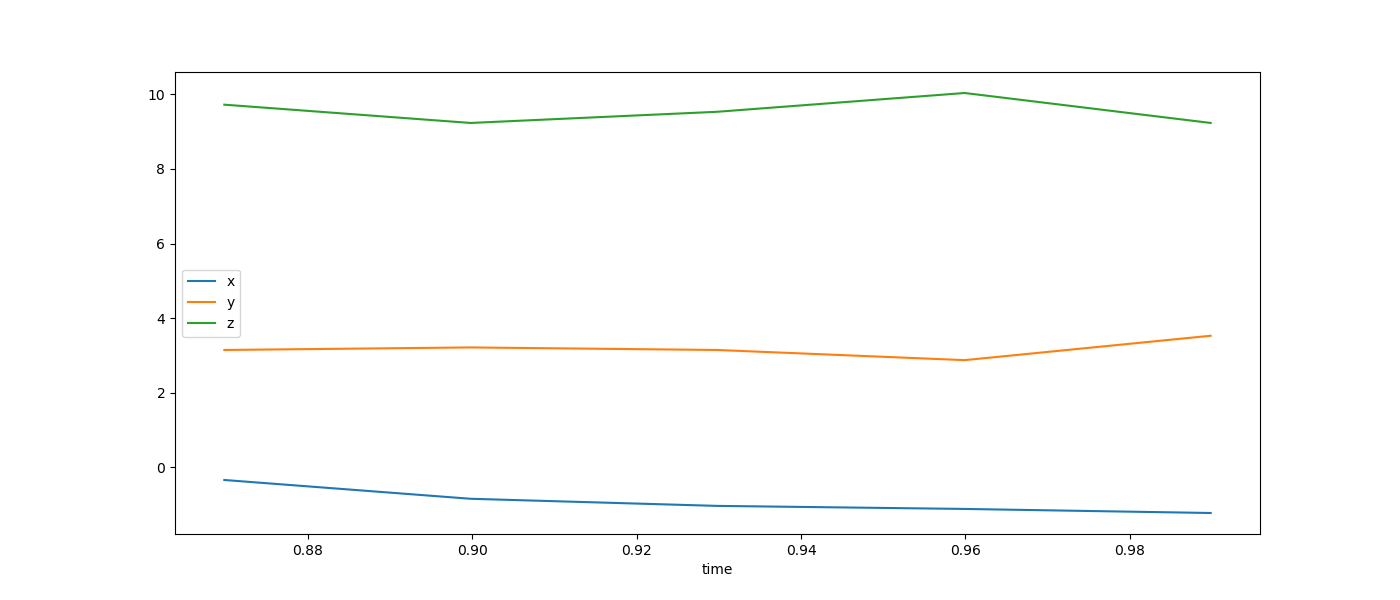
To plot the data in our data window, we can just call the plot method on it.
In [39]: w_data.plot('time', ['x', 'y', 'z'], figsize=(14,6))
Out[39]: <matplotlib.axes._subplots.AxesSubplot at 0x1fc7fbd02e8>
Building Projects Programmatically
In addition to loading projects from XML definitions, you can create and edit
projects programmatically. To create a new Project object, you would
do the following:
In [40]: kmeans = conn.create_project('kmeans')

Adding a Data Window
We now need to add a source window for the data. All window objects are created from the ESP connection. This is due to the fact that some of the window classes are generated based on extensions installed in the server.
First we create a window object:
In [41]: dataw = conn.SourceWindow(schema=('id*:int64', 'x_c:double', 'y_c:double'),
   ....:                           insert_only=True)
   ....:
Now we can add that window to our project:
In [42]: kmeans.windows['dataw'] = dataw

Adding a Training Window
Now that we have a way to get data into the project, let’s add a training window using the KMEANS algorithm. The first argument is the name of the window in the project. The keyword arguments are various parameters used to modify the training algorithm.
These parameters are descrbed in the documentation string of the KMEANS
class. To see what they all do, use help(conn.train.KMEANS).
In [43]: train = conn.train.KMEANS(
   ....:     velocity=5, fadeOutFactor=0.05, nClusters=2, dampingFactor=0.8,
   ....:     nInit=50, commitInterval=25, initSeed=1, disturbFactor=0.01
   ....: )
   ....:
We can now set additional attributes on the window such as the input map variables.
In [44]: train.set_inputs(inputs=('x_c', 'y_c'))
With the window fully configured, we can add it to our project.
In [45]: kmeans.windows['train_kmeans'] = train

Adding a Scoring Window
With the training window in place, we can now add a scoring window.
In [46]: score = conn.score.KMEANS(schema=('id*:int64', 'x_c:double', 'y_c:double',
   ....:                                   'min_dist:double', 'seg:int32', 'model_id:int64'))
   ....:

In [47]: score.set_outputs(minDistanceOut='min_dist',
   ....:                   labelOut='seg',
   ....:                   modelIdOut='model_id')
   ....:

In [48]: kmeans.windows['score_kmeans'] = score
In this window, we must add a model and set the output variable names for the
variables that are computed. Again, you can use help(conn.score.KMEANS)
to see what the output variables are.
Making Connections between Windows
Now that we have all of our windows created, we need to connect them. This is what the project looks like now.

To connect windows, we use the add_target() method.
In [49]: dataw.add_target(train, role='data')

In [50]: dataw.add_target(score, role='data')

In [51]: train.add_target(score, role='model')

Loading the Project into the Server
Now that we have our project completed, we can load it into the server using
the load_project() method.
In [52]: conn.load_project(kmeans)
Out[52]: Project(name='kmeans')
We can get the current projects to verify that it has been loaded.
In [53]: conn.get_projects()
Out[53]: {'kmeans': Project(name='kmeans'), 'project': Project(name='project')}
Publishing Events to Data Window
We can now publish events to the data window and set the whole project into motion. Here is the data, we will be injecting.
In [54]: kmeans_csv = '''
   ....:     0,0.5908967210216602,1.6751986326790076
   ....:     1,19.043415721883388,18.371355627504236
   ....:     2,-0.012273367464207865,-0.4540492269435668
   ....:     3,17.97874517980503,21.65120582597203
   ....:     4,1.1659924204397523,-1.2409508065225885
   ....:     5,0.8546216190275081,-0.25882119862607184
   ....:     6,20.190217162336587,22.50997309914134
   ....:     7,-0.25895458090747875,1.4976085871983391
   ....:     8,22.29022654822051,16.914962015510373
   ....:     9,20.77677573497869,19.816778938696523
   ....:     10,20.325394323107314,19.87786781139061
   ....:     11,17.92502239930997,20.062599670620752
   ....:     12,-1.1833277290532713,0.7203950672666275
   ....:     13,3.126014444864653,8.954400059737004
   ....:     14,1.1893660438670264,-2.0446842195717476
   ....:     15,20.120414292371407,20.146941695024136
   ....:     16,0.4917130506091213,-0.784642721030343
   ....:     17,0.22291063630044675,-0.41514920558560614
   ....:     18,2.8717071803941447,-1.6159246657278439
   ....:     19,-0.45380722464073486,-0.4407066391442154
   ....:     20,0.6149331209790688,1.522123705249856
   ....:     21,19.84694537818082,19.702918586896455
   ....:     22,16.436483339375265,20.804351101633195
   ....:     23,-0.8167794351602463,-0.723820028820651
   ....:     24,20.65091100640363,21.608200883324137
   ....:     25,19.140236340468213,20.82808262209404
   ....:     26,-0.4875727732042338,0.747112259920503
   ....:     27,20.4113258319396,18.766159688735634
   ....:     28,0.2537975739650817,0.36373384398482916
   ....:     29,20.695390556004522,19.774253133582604
   ....:     30,18.28928467597047,21.516368054185115
   ....:     31,19.978643758572222,20.785814123577413
   ....:     32,19.04110630167857,19.05452162304791
   ....:     33,2.661387735425831,-1.1899037392988199
   ....:     34,19.382293352002982,19.56970305958366
   ....:     35,19.637004907161717,20.72555629061505
   ....:     36,20.818644254655087,17.93507500279616
   ....:     37,18.8471473497551,19.226894183030726
   ....:     38,3.565412061996094,6.054056158175342
   ....:     39,20.08998741404671,20.355429746977276
   ....:     40,-2.666446517271164,-1.4728455045410282
   ....:     41,19.149653728344884,21.216873467449357
   ....:     42,2.1331364719647166,0.22833700336859286
   ....:     43,1.7522057911939954,-0.03250537224830827
   ....:     44,20.786846005628114,20.160909258507722
   ....:     45,-3.0032525575973525,-0.47164367434522386
   ....:     46,2.279071289695989,0.25303073769270384
   ....:     47,1.8510594272972942,-2.3126288328396645
   ....:     48,-1.692179065795689,-3.067171903045865
   ....:     49,-0.10268366234705945,-0.7786701219856643
   ....:     50,20.39050392631347,20.5343519173733
   ....:     51,-1.218501669497454,-2.952991443676715
   ....:     52,1.254811095346156,0.2590241868676189
   ....:     53,1.7994383767768294,-2.0499967578177785
   ....:     54,20.029238232230277,22.914597444964127
   ....:     55,1.7589545563883249,1.0376747852275094
   ....:     56,-0.39993518183515325,-1.1657700593370808
   ....:     57,-0.22788200103761708,1.2574585872035329
   ....:     58,-8.321390217413192,-4.328504673489415
   ....:     59,0.33948826344937444,-0.08069060680732133
   ....:     60,1.4957191917037937,-1.1193342088301603
   ....: '''
   ....:
We will again use the publish_events() method to send the data
to the server. In this case, we’ll use a 200 millisecond event rate.
In [55]: dataw.publish_events(kmeans_csv, pause=200)

In [56]: dataw.subscribe()

In [57]: score.subscribe()
We can then see the data flowing through the data and score windows.
In [58]: print(dataw)
          x_c        y_c
id
1   19.043416  18.371356
2   -0.012273  -0.454049
3   17.978745  21.651206
4    1.165992  -1.240951
5    0.854622  -0.258821
6   20.190217  22.509973
7   -0.258955   1.497609
8   22.290227  16.914962
9   20.776776  19.816779
10  20.325394  19.877868
11  17.925022  20.062600
12  -1.183328   0.720395
13   3.126014   8.954400
14   1.189366  -2.044684
15  20.120414  20.146942
16   0.491713  -0.784643
17   0.222911  -0.415149
18   2.871707  -1.615925
19  -0.453807  -0.440707
20   0.614933   1.522124
21  19.846945  19.702919
22  16.436483  20.804351
23  -0.816779  -0.723820
24  20.650911  21.608201
25  19.140236  20.828083
26  -0.487573   0.747112
27  20.411326  18.766160
28   0.253798   0.363734
29  20.695391  19.774253
30  18.289285  21.516368
31  19.978644  20.785814
32  19.041106  19.054522
33   2.661388  -1.189904
34  19.382293  19.569703
35  19.637005  20.725556
36  20.818644  17.935075
37  18.847147  19.226894
38   3.565412   6.054056
39  20.089987  20.355430
40  -2.666447  -1.472846
41  19.149654  21.216873
42   2.133136   0.228337
43   1.752206  -0.032505
44  20.786846  20.160909
45  -3.003253  -0.471644
46   2.279071   0.253031
47   1.851059  -2.312629
48  -1.692179  -3.067172
49  -0.102684  -0.778670
50  20.390504  20.534352
51  -1.218502  -2.952991

In [59]: print(score)
         x_c        y_c   min_dist  seg  model_id
id
50  20.390504  20.534352  11.498755    1         0
51  -1.218502  -2.952991  11.705346    0         0
Conclusion
We have covered the basics of connecting to ESP, getting information from the server, and working with projects here. The API Reference contains the complete information about what methods and attributes are available on all of the objects touched on here, as well as many others.